Endogeneity occurs when it is impossible to establish a chain of causality among variables. An instance of this might be AIDS funding in Uganda and AIDS occurence in Uganda. The problem here is that the amount of funding is a function of the number of AIDS cases in Uganda, however the number of cases is also affected by funding - what came first, chicken or the egg?
In this notebook I use a fertility data set to explore factors that might affect the age of a woman when she has her first child. The data is from James Heakins, a former undergraduate student of Professor Wooldridge at Michigan State University, for a term project. They come from Botswana’s 1988 Demographic and Health Survey.
Here’s my roadmap for evaluating this data:
- I begin by looking at some scatterplots of the variables so that I can begin to get an idea of their relationship to one another.
- Estimate a naive equation with a possibly endogenous variable. The dependent variable will always be age at first birth.
- Identify the endogenous variable and pick an appropiate instrument for it. Test for the relevancy of this instrument using an f-test.
- Use 2-stage least squares regression to estimate a new OLS model with the proper instrument included. I use IV2SLS written by the wonderful people at statsmodels.
- As an exercise, replicate part 4 using matrix algebra in Numpy
- Test for exogeneity of (supposedly) endogenous variable using the Hausman-Wu test.
- Add another instrument to the mix, repeat step 3 for both instruments.
- Test for overidentification using the Sagan test.
import pandas as pd
import numpy as np
import statsmodels.api as sm
from statsmodels.sandbox.regression.gmm import IV2SLS
from __future__ import division
import seaborn as sns

%matplotlib inline
import matplotlib.pylab as plt
from matplotlib.pylab import rcParams
rcParams['figure.figsize'] = 18.5, 10.5

def print_resids(preds, resids):
    ax = sns.regplot(preds, resids);
    ax.set(xlabel = 'Predicted values', ylabel = 'errors', title = 'Predicted values vs. Errors')
    plt.show();
Part 1
Load data, do some exploration on it
fertility = pd.read_stata("http://rlhick.people.wm.edu/econ407/data/fertility.dta")
fertility.shape
(4361, 27)
Take a peek at the relationship between education and age of first birth, as well as the number of children and age of first birth.
fertility.plot.scatter('educ', 'agefbrth'); fertility.plot.scatter( 'agefbrth', 'children');
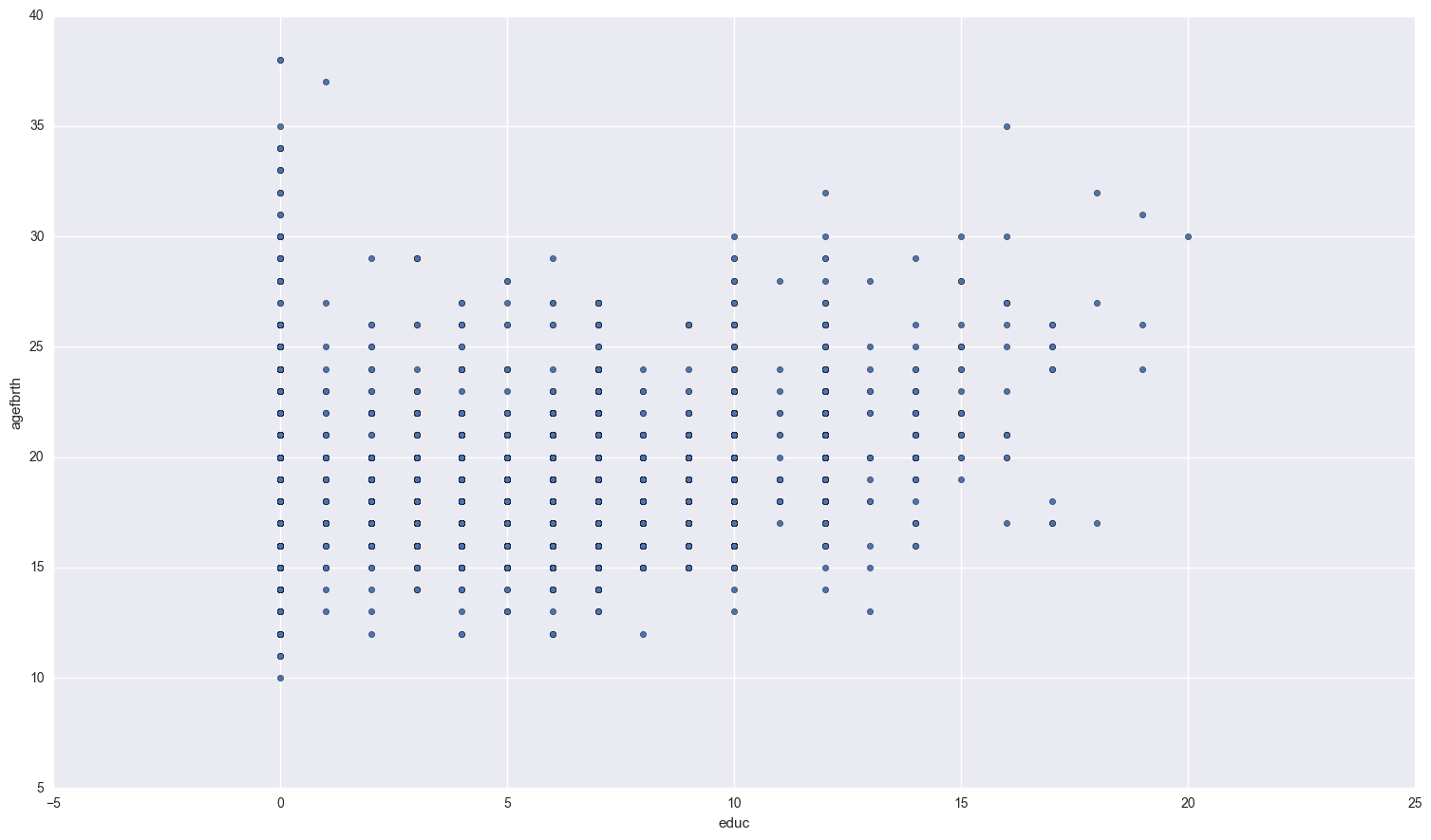
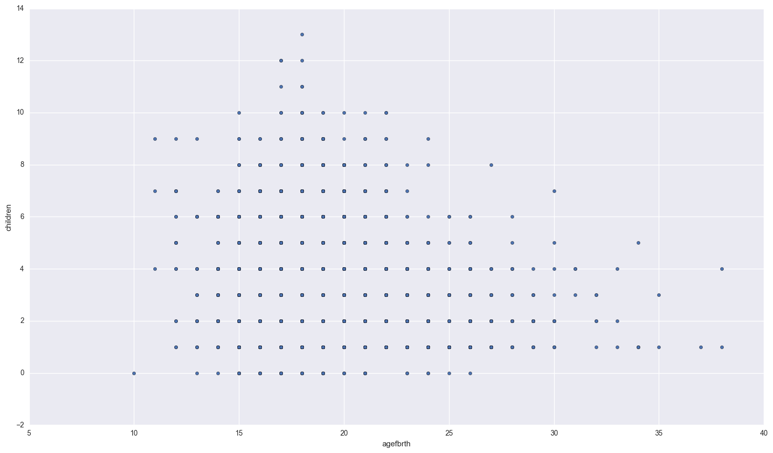
If you squint a bit, there seems to be a small positive relationship between how much education a woman recieves and the age of her first birth. As for the relationship between age of first birth and total number of children, women who have their first child at a young age seem to have more children overall.
Lets compare the first birth age of women who use a method of contraception to those who don’t.
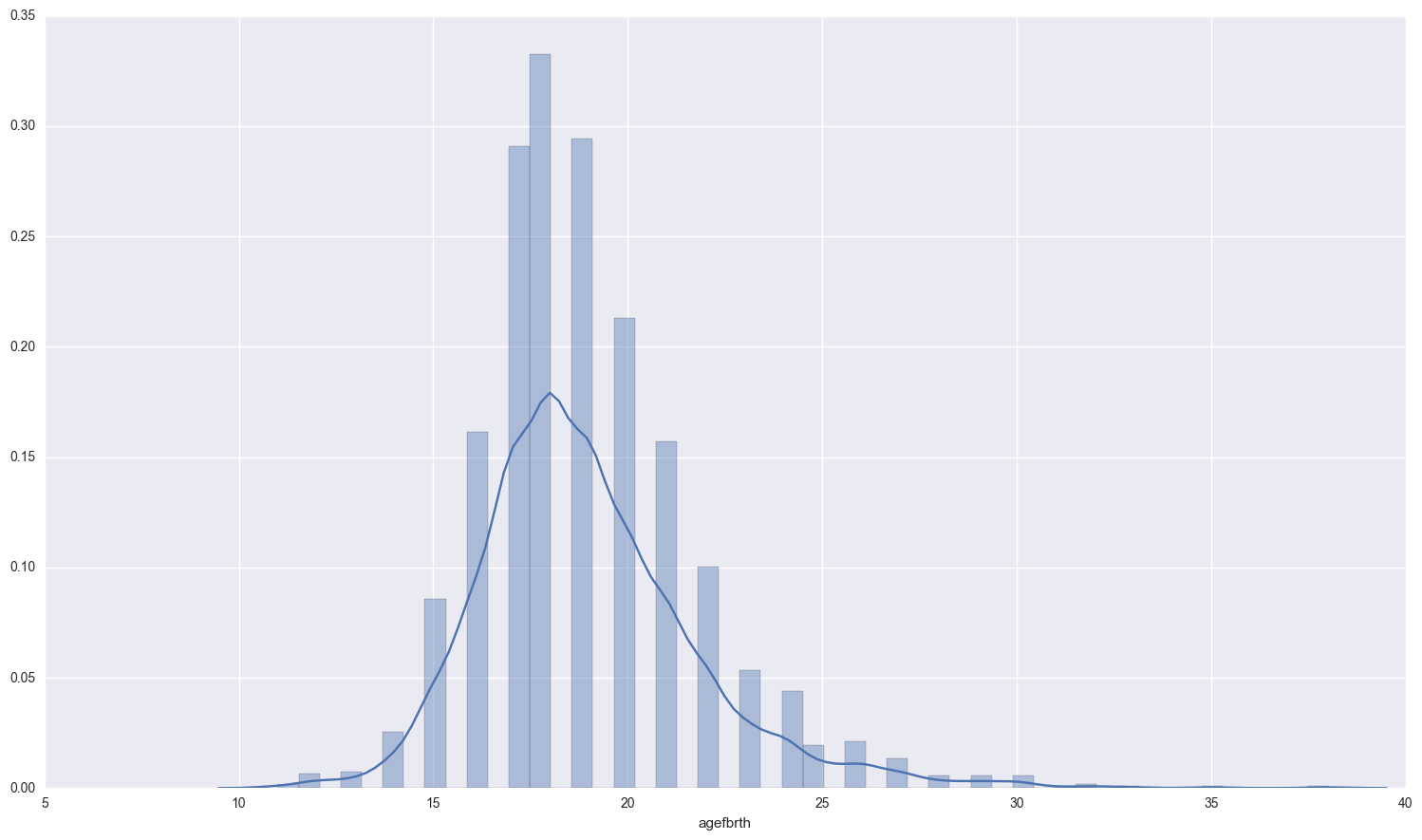
These women have used a method of birth control at least once:
print fertility[fertility['usemeth'] == 1]['agefbrth'].dropna().describe()
sns.distplot(fertility[fertility['usemeth'] == 1]['agefbrth'].dropna() );
count    2182.000000
mean       18.952795
std         2.834758
min        11.000000
25%        17.000000
50%        19.000000
75%        20.000000
max        38.000000
Name: agefbrth, dtype: float64
These women have never used any method of birth control:
print fertility[fertility['usemeth'] == 0]['agefbrth'].dropna().describe()
sns.distplot(fertility[fertility['usemeth'] == 0]['agefbrth'].dropna() );
count    1031.000000
mean       19.115421
std         3.591423
min        10.000000
25%        17.000000
50%        19.000000
75%        21.000000
max        38.000000
Name: agefbrth, dtype: float64
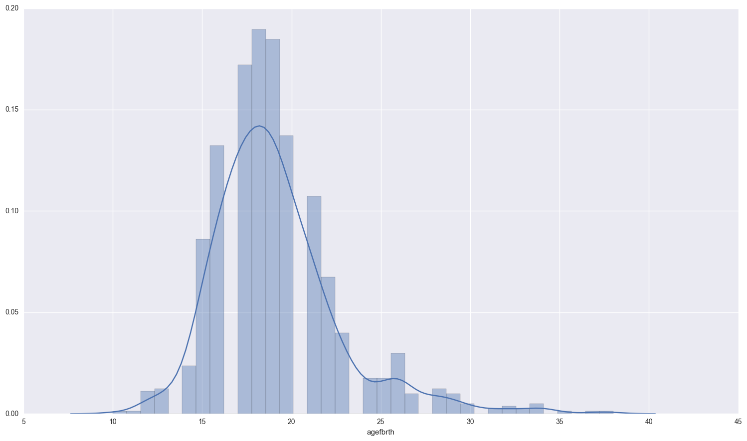
Somewhat interesting… the mean age of 1st birth for women who have ever used a method of birth control is lower than those that have never used one. However, there is slightly more variation in the women who don’t use birth control.
Part 2
estimate naive equation with a possibly endogenous variable
The equation I will estimate is:
We assume that there is no relationship between education and the number of children ever born or education and month of marriage. We also assume that there is no relationship between month of first marriage and number of children born.
Theres a huge problem with missing data in this dataset, roughly a half of agefbrth data a missing from the total amount of observations. I get rid of the data now that has null values for age of first birth, education, month of first marriage, and children ever born.
#gets all columns that aren't null
no_null = fertility[(fertility['agefbrth'].notnull()) & (fertility['educ'].notnull()) &
                    (fertility.monthfm.notnull()) & (fertility['ceb'].notnull()) & (fertility['idlnchld'].notnull())]

print "lost {} samples of data out of a total {} samples".format(fertility.shape[0] - no_null.shape[0],
                                                                 fertility.shape[0] )

ind_vars = ['monthfm', 'ceb', 'educ', 'idlnchld']
dep_var = 'agefbrth'
x = no_null[ind_vars]
y = no_null[dep_var]

x_const = sm.add_constant(x)

first_model_results = sm.OLS(y, x_const, missing = 'drop').fit()

#results = first_model.fit()

first_model_results.summary()
lost 2489 samples of data out of a total 4361 samples
| Dep. Variable: | agefbrth | R-squared: | 0.058 |
|---|---|---|---|
| Model: | OLS | Adj. R-squared: | 0.056 |
| Method: | Least Squares | F-statistic: | 28.83 |
| Date: | Sun, 15 Jan 2017 | Prob (F-statistic): | 2.78e-23 |
| Time: | 15:51:50 | Log-Likelihood: | -4811.1 |
| No. Observations: | 1872 | AIC: | 9632. |
| Df Residuals: | 1867 | BIC: | 9660. |
| Df Model: | 4 | ||
| Covariance Type: | nonrobust |
| coef | std err | t | P>|t| | [95.0% Conf. Int.] | |
|---|---|---|---|---|---|
| const | 18.9236 | 0.294 | 64.289 | 0.000 | 18.346 19.501 |
| monthfm | 0.0413 | 0.020 | 2.043 | 0.041 | 0.002 0.081 |
| ceb | -0.1588 | 0.034 | -4.640 | 0.000 | -0.226 -0.092 |
| educ | 0.1303 | 0.019 | 6.830 | 0.000 | 0.093 0.168 |
| idlnchld | -0.0101 | 0.034 | -0.298 | 0.766 | -0.077 0.056 |
| Omnibus: | 508.807 | Durbin-Watson: | 1.920 |
|---|---|---|---|
| Prob(Omnibus): | 0.000 | Jarque-Bera (JB): | 1674.738 |
| Skew: | 1.339 | Prob(JB): | 0.00 |
| Kurtosis: | 6.781 | Cond. No. | 43.9 |
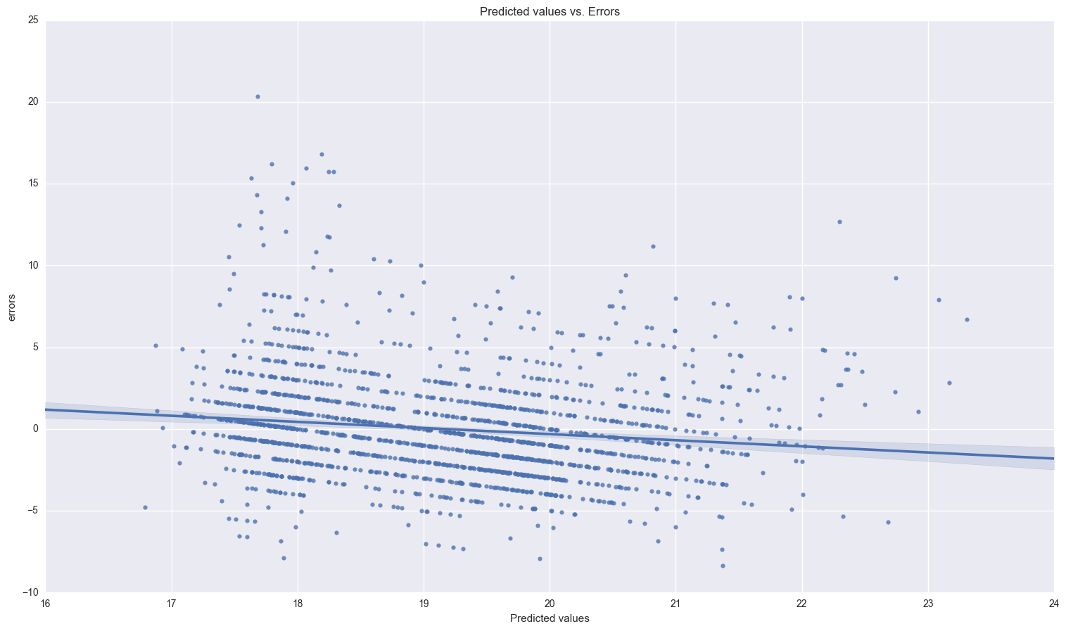
print_resids(first_model_results.predict(x_const), first_model_results.resid)
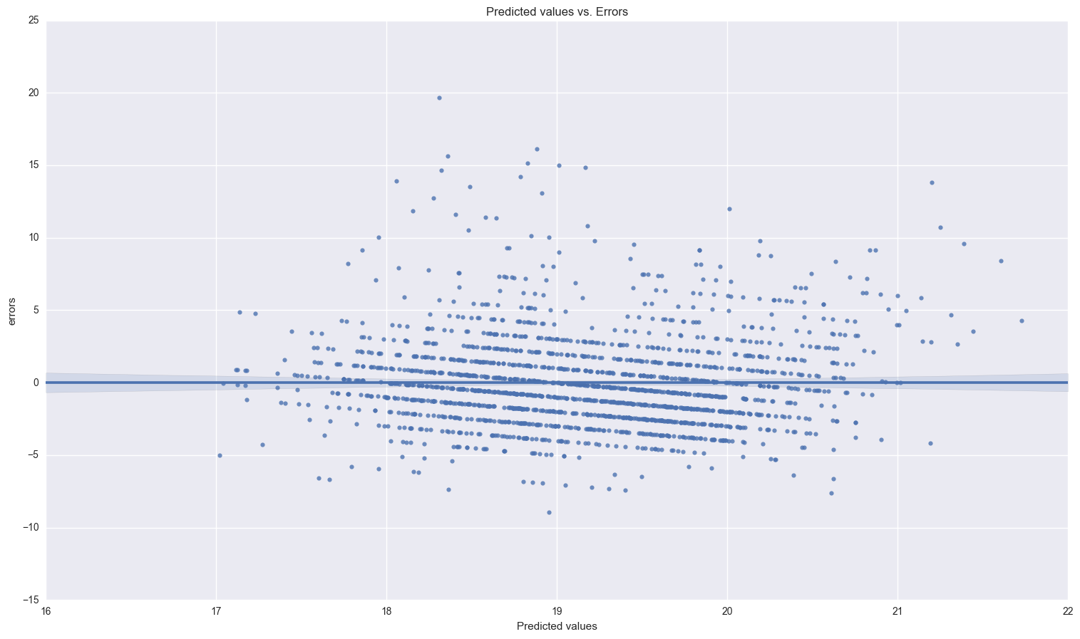
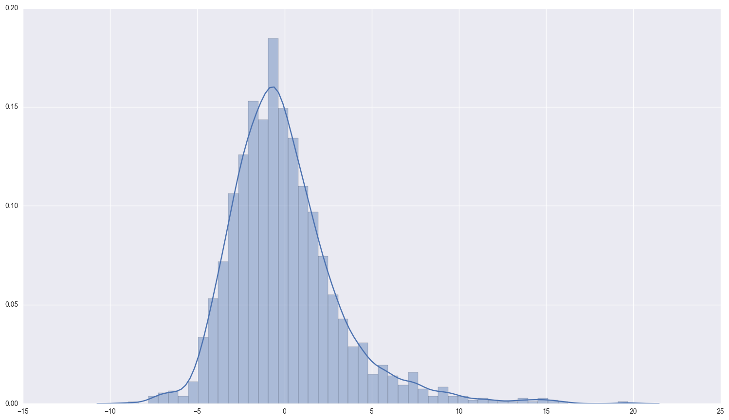
print "the descriptive statistics for the errors and a histogram of them:\n\n", first_model_results.resid.describe()
sns.distplot(first_model_results.resid);
the descriptive statistics for the errors and a histogram of them:

count    1872.000000
mean       -0.000002
std         3.162461
min        -8.951200
25%        -2.016429
50%        -0.468160
75%         1.414013
max        19.689455
dtype: float64
There’s definitely some linear structure to the errors here, caused by the discrete nature of the dependent variable. (Maybe build a classification model for this?)
The exogeneity assumptions are not valid here. It’s reasonable to believe that amount of education recieved is correlated with errors in age of first birth. Education and the month of the first marriage are possibly weakly related. I’m not sure how the school years in Botswana are structured, but if a woman is in school for part of a year, she may not want to get married during any of those months, thus affecting the month she is married. We proceed with caution.
Part 3: Pick an instrument and test for relevancy and strength
I hypothesize that the most endogenous variable is education. If a child is born at a young age, there is less time for education, and it is impossible to determine which is the causal variable.
I will use electricity as an instrumental variable. There is no reason to believe that errors in age of birth and electricity are directly related to each other. However, education and electricity are probably related because places that have electricity are probably more developed and thus more likely to have a school. So, electricity is related to age of first birth only via education.
test for the relevancy of electricity as an instrumental variable:
- run relevancy equation where exogenous variables and instrument predict the endogenous variable.
- test whether the coefficient on the instrument is 0 via an F-test with one degree of freedom
rel = ['monthfm', 'ceb', 'electric']
endog = 'educ'

dropped_na = fertility[(fertility.monthfm.notnull()) & (fertility.ceb.notnull()) & (fertility.electric.notnull())
                    & (fertility.educ.notnull())]

only_exog = sm.add_constant(dropped_na[rel])
relevancy_results = sm.OLS(dropped_na[endog], only_exog).fit()

relevancy_results.summary()
| Dep. Variable: | educ | R-squared: | 0.269 |
|---|---|---|---|
| Model: | OLS | Adj. R-squared: | 0.268 |
| Method: | Least Squares | F-statistic: | 253.9 |
| Date: | Sun, 15 Jan 2017 | Prob (F-statistic): | 2.70e-140 |
| Time: | 15:51:53 | Log-Likelihood: | -5605.4 |
| No. Observations: | 2076 | AIC: | 1.122e+04 |
| Df Residuals: | 2072 | BIC: | 1.124e+04 |
| Df Model: | 3 | ||
| Covariance Type: | nonrobust |
| coef | std err | t | P>|t| | [95.0% Conf. Int.] | |
|---|---|---|---|---|---|
| const | 5.7469 | 0.205 | 27.973 | 0.000 | 5.344 6.150 |
| monthfm | 0.0220 | 0.022 | 1.007 | 0.314 | -0.021 0.065 |
| ceb | -0.4456 | 0.032 | -13.811 | 0.000 | -0.509 -0.382 |
| electric | 4.6753 | 0.216 | 21.634 | 0.000 | 4.251 5.099 |
| Omnibus: | 38.041 | Durbin-Watson: | 1.527 |
|---|---|---|---|
| Prob(Omnibus): | 0.000 | Jarque-Bera (JB): | 23.335 |
| Skew: | 0.100 | Prob(JB): | 8.57e-06 |
| Kurtosis: | 2.521 | Cond. No. | 24.4 |
Run the hypothesis test that the coefficient on electric is 0:
this is where I found this test
hypothesis = '(electric = 0)'
print relevancy_results.f_test(hypothesis)
<F test: F=array([[ 468.01322886]]), p=9.5448237988e-94, df_denom=2072, df_num=1>
With an F-statistic of 440.417, this is surely a relevant and strong instrument. The F-statistic must be at least 10 in order to be a strong instrument.
Part 4: Instrumenting using two-stage least squares
Some background and information about two-stage least squares regression: It’s called two stage because there are actually two stages of regression done (earth shattering I know).
First stage
In the first stage, the matrix $X$, which contains the endogenous information, is projected on to $Z$. $Z$ is the matrix without endogenous information that includes the variable(s) that are our instruments. Mathematically: where $V$ is the error, and $\hat\gamma = (Z’ Z)^{-1}Z’ X$.
The projection of X on to Z is then:
Second stage
We repeat the same process as above using
Specifying the two stage least squares model
The documentation for IV2SLS in statsmodels is somewhat confusing and conflicts with some of the terminology that I’ve used in my classes. So, for clarification:
- endog is the dependent variable, y
- exog is the x matrix that has the endogenous information in it. Include the endogenous variables in it.
- instrument is the z matrix. Include all the variables that are not endogenous and replace the endogenous variables from the exog matrix (above) with what ever instruments you choose for them.
no_null_iv = fertility[(fertility['agefbrth'].notnull()) & (fertility['electric'].notnull()) &
                    (fertility['monthfm'].notnull()) & (fertility['ceb'].notnull()) & (fertility['educ'].notnull())
                      & (fertility['idlnchld'].notnull())]
endog = no_null_iv['agefbrth']
exog = no_null_iv[['monthfm', 'ceb', 'idlnchld', 'educ']]
instr = no_null_iv[['monthfm', 'ceb', 'idlnchld', 'electric']]
dep_var_iv = no_null_iv['agefbrth']

exog_constant = sm.add_constant(exog)
instr_constant = sm.add_constant(instr)
no_endog_results = IV2SLS(endog, exog_constant, instrument = instr_constant).fit()

no_endog_results.summary()
| Dep. Variable: | agefbrth | R-squared: | 0.005 |
|---|---|---|---|
| Model: | IV2SLS | Adj. R-squared: | 0.003 |
| Method: | Two Stage | F-statistic: | 28.06 |
| Least Squares | Prob (F-statistic): | 1.16e-22 | |
| Date: | Sun, 15 Jan 2017 | ||
| Time: | 15:51:56 | ||
| No. Observations: | 1870 | ||
| Df Residuals: | 1865 | ||
| Df Model: | 4 |
| coef | std err | t | P>|t| | [95.0% Conf. Int.] | |
|---|---|---|---|---|---|
| const | 17.0973 | 0.507 | 33.696 | 0.000 | 16.102 18.092 |
| monthfm | 0.0411 | 0.021 | 1.973 | 0.049 | 0.000 0.082 |
| ceb | -0.0635 | 0.041 | -1.540 | 0.124 | -0.144 0.017 |
| idlnchld | 0.0780 | 0.040 | 1.949 | 0.051 | -0.000 0.156 |
| educ | 0.3276 | 0.048 | 6.829 | 0.000 | 0.234 0.422 |
| Omnibus: | 530.134 | Durbin-Watson: | 1.907 |
|---|---|---|---|
| Prob(Omnibus): | 0.000 | Jarque-Bera (JB): | 1901.731 |
| Skew: | 1.366 | Prob(JB): | 0.00 |
| Kurtosis: | 7.116 | Cond. No. | 43.8 |
The effect of education on the age of first birth is fairly large.
On average, every year of education increases age of first birth by .327 years. This speaks to the positive effects of education. Interestingly, it is the only statistically significant variable at the .01 level.
print_resids(no_endog_results.predict(), no_endog_results.resid)
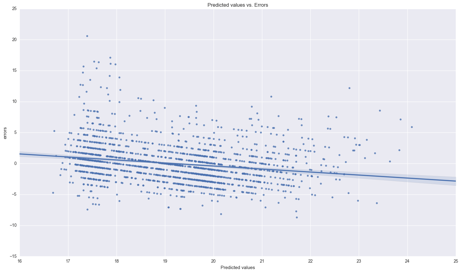
print "the descriptive statistics for the errors and a histogram of them:\n\n", no_endog_results.resid.describe()
sns.distplot(no_endog_results.resid);
the descriptive statistics for the errors and a histogram of them:

count    1.870000e+03
mean    -7.649794e-07
std      3.252076e+00
min     -8.714241e+00
25%     -2.057206e+00
50%     -4.409256e-01
75%      1.484385e+00
max      2.060653e+01
dtype: float64
Part 5: replicate using matrix algebra
first, replicate OLS estimates:
x_mat_ols = np.matrix(x_const)
y_mat_ols = np.matrix(y)
y_mat_ols = np.reshape(y_mat_ols, (-1, 1)) #reshape so that its a single column vector, not row vector
b_ols = np.linalg.inv(x_mat_ols.T*x_mat_ols)*x_mat_ols.T*y_mat_ols
print b_ols
[[  1.89236317e+01]
 [  4.13089916e-02]
 [ -1.58784062e-01]
 [  1.30279362e-01]
 [ -1.00923479e-02]]
those check out with our original naive estimates with endogeneity.
Now, the IV estimates, using the z-matrix:
y_iv_mat = np.matrix(endog)
y_iv_mat = np.reshape(y_iv_mat, (-1, 1))
z_mat = np.matrix(instr_constant)
x_mat_iv = np.matrix(exog_constant)
np.linalg.inv(z_mat.T * x_mat_iv)*z_mat.T*y_iv_mat
matrix([[ 17.09725189],
        [  0.04106776],
        [ -0.06348502],
        [  0.07799444],
        [  0.32765239]], dtype=float32)
Yay, everything checks out! For clarity, the z matrix only contains exogenous information, while x constains our endogenous variable education.
Part 6: Hausman-Wu test for endogeneity
Steps:
- Run relevancy regression (endog variable ~ exogenous variables + instrument(s) + error)
- Get the predicted residuals from this regression ($\hat r$)
- Run regression $Y = X\gamma + \hat r \beta + u$
- Test whether the coefficient on $\hat r$ is significantly different than 0 using an F-test with 1 degree of freedom
# add relevancy equation residuals on to the endogenous matrix
x_const['relevancy_resids'] = relevancy_results.resid

# run endogenous regression now with residuals added in
endog_test_results = sm.OLS(y, x_const, missing = 'drop').fit()

endog_test_results.summary()
| Dep. Variable: | agefbrth | R-squared: | 0.069 |
|---|---|---|---|
| Model: | OLS | Adj. R-squared: | 0.067 |
| Method: | Least Squares | F-statistic: | 27.83 |
| Date: | Sun, 15 Jan 2017 | Prob (F-statistic): | 2.91e-27 |
| Time: | 15:51:59 | Log-Likelihood: | -4795.4 |
| No. Observations: | 1870 | AIC: | 9603. |
| Df Residuals: | 1864 | BIC: | 9636. |
| Df Model: | 5 | ||
| Covariance Type: | nonrobust |
| coef | std err | t | P>|t| | [95.0% Conf. Int.] | |
|---|---|---|---|---|---|
| const | 17.6155 | 0.407 | 43.296 | 0.000 | 16.818 18.413 |
| monthfm | 0.0412 | 0.020 | 2.047 | 0.041 | 0.002 0.081 |
| ceb | -0.0618 | 0.040 | -1.541 | 0.123 | -0.140 0.017 |
| educ | 0.3102 | 0.043 | 7.213 | 0.000 | 0.226 0.394 |
| idlnchld | -0.0005 | 0.034 | -0.014 | 0.989 | -0.067 0.066 |
| relevancy_resids | -0.2192 | 0.047 | -4.654 | 0.000 | -0.312 -0.127 |
| Omnibus: | 494.869 | Durbin-Watson: | 1.931 |
|---|---|---|---|
| Prob(Omnibus): | 0.000 | Jarque-Bera (JB): | 1630.863 |
| Skew: | 1.302 | Prob(JB): | 0.00 |
| Kurtosis: | 6.761 | Cond. No. | 61.3 |
null_hypothesis = '(relevancy_resids = 0)'
print endog_test_results.f_test(null_hypothesis)
<F test: F=array([[ 21.65873982]]), p=3.48680999408e-06, df_denom=1864, df_num=1>
We reject the null hypothesis that education is exogenous and conclude that education is indeed an endogenous variable.
The thinking behind this test is that the residuals should only include endogenous information of education because we explained all the exogenous information with monthfm and ceb. If we can then use that endogenous information to predict y in a meaningful way (i.e. the coefficient isn’t zero), then that is evidence that education is correlated with age of first birth via the error term.
Part 7: Add another instrument
Now we instrument for education using more than one instrumental variable. Living in an urban area should not be related to differences in the age of first birth, however, it will affect educational attainment. Again, more developed areas should (presumably) have better access to schools and education.
two_ivs = fertility[(fertility['agefbrth'].notnull()) & (fertility['electric'].notnull()) &
                    (fertility['monthfm'].notnull()) & (fertility['ceb'].notnull()) & (fertility['educ'].notnull())
                      & (fertility['idlnchld'].notnull()) & (fertility['urban'].notnull())]

endog = two_ivs['agefbrth']
exog = two_ivs[['monthfm', 'ceb', 'idlnchld', 'educ']]
instr = two_ivs[['monthfm', 'ceb', 'idlnchld', 'electric', 'urban']]


exog_constant = sm.add_constant(exog)
instr_constant = sm.add_constant(instr)
two_iv_results = IV2SLS(endog, exog_constant, instrument = instr_constant).fit()

two_iv_results.summary()
| Dep. Variable: | agefbrth | R-squared: | 0.033 |
|---|---|---|---|
| Model: | IV2SLS | Adj. R-squared: | 0.031 |
| Method: | Two Stage | F-statistic: | 25.28 |
| Least Squares | Prob (F-statistic): | 2.01e-20 | |
| Date: | Sun, 15 Jan 2017 | ||
| Time: | 15:52:03 | ||
| No. Observations: | 1870 | ||
| Df Residuals: | 1865 | ||
| Df Model: | 4 |
| coef | std err | t | P>|t| | [95.0% Conf. Int.] | |
|---|---|---|---|---|---|
| const | 17.6755 | 0.488 | 36.215 | 0.000 | 16.718 18.633 |
| monthfm | 0.0412 | 0.021 | 2.011 | 0.044 | 0.001 0.081 |
| ceb | -0.0939 | 0.040 | -2.335 | 0.020 | -0.173 -0.015 |
| idlnchld | 0.0501 | 0.039 | 1.281 | 0.200 | -0.027 0.127 |
| educ | 0.2655 | 0.046 | 5.795 | 0.000 | 0.176 0.355 |
| Omnibus: | 531.978 | Durbin-Watson: | 1.918 |
|---|---|---|---|
| Prob(Omnibus): | 0.000 | Jarque-Bera (JB): | 1891.653 |
| Skew: | 1.374 | Prob(JB): | 0.00 |
| Kurtosis: | 7.089 | Cond. No. | 43.8 |
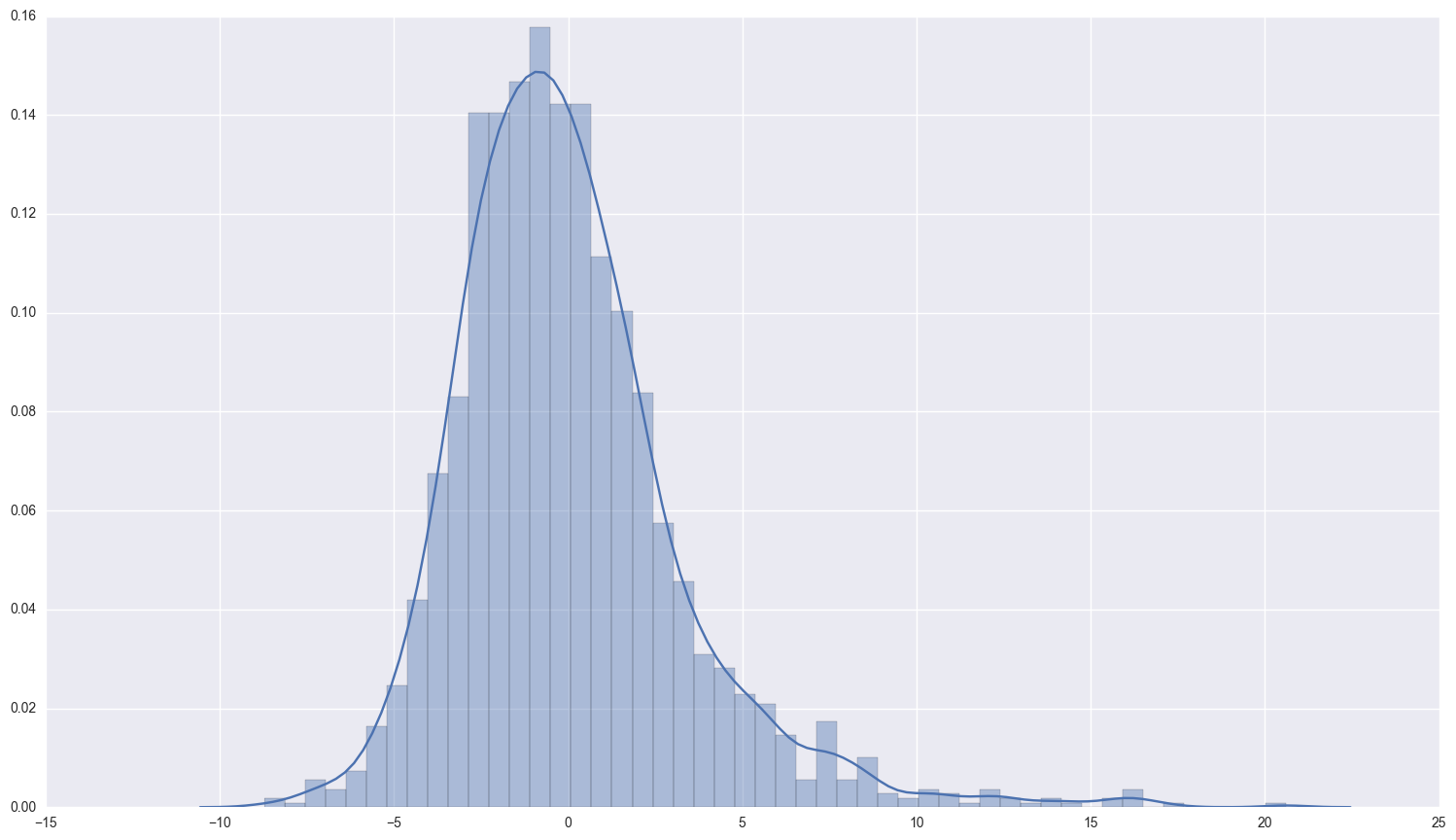
print_resids(two_iv_results.predict(), two_iv_results.resid)
print two_iv_results.resid.describe()
sns.distplot(two_iv_results.resid);
count    1.870000e+03
mean     2.600930e-07
std      3.204986e+00
min     -8.368925e+00
25%     -2.044604e+00
50%     -4.985476e-01
75%      1.411119e+00
max      2.031738e+01
dtype: float64

Now, we test for the relevancy and strength of our instruments:
rel = ['monthfm', 'ceb', 'electric', 'urban']
endog = 'educ'

only_exog = sm.add_constant(fertility[rel])
relevancy_results = sm.OLS(fertility[endog], only_exog, missing = 'drop').fit()

relevancy_results.summary()
| Dep. Variable: | educ | R-squared: | 0.281 |
|---|---|---|---|
| Model: | OLS | Adj. R-squared: | 0.280 |
| Method: | Least Squares | F-statistic: | 202.7 |
| Date: | Sun, 15 Jan 2017 | Prob (F-statistic): | 7.76e-147 |
| Time: | 15:52:06 | Log-Likelihood: | -5587.4 |
| No. Observations: | 2076 | AIC: | 1.118e+04 |
| Df Residuals: | 2071 | BIC: | 1.121e+04 |
| Df Model: | 4 | ||
| Covariance Type: | nonrobust |
| coef | std err | t | P>|t| | [95.0% Conf. Int.] | |
|---|---|---|---|---|---|
| const | 5.1261 | 0.228 | 22.450 | 0.000 | 4.678 5.574 |
| monthfm | 0.0247 | 0.022 | 1.137 | 0.255 | -0.018 0.067 |
| ceb | -0.4105 | 0.033 | -12.626 | 0.000 | -0.474 -0.347 |
| electric | 4.2665 | 0.225 | 18.979 | 0.000 | 3.826 4.707 |
| urban | 1.0167 | 0.169 | 6.019 | 0.000 | 0.685 1.348 |
| Omnibus: | 32.600 | Durbin-Watson: | 1.546 |
|---|---|---|---|
| Prob(Omnibus): | 0.000 | Jarque-Bera (JB): | 21.735 |
| Skew: | 0.118 | Prob(JB): | 1.91e-05 |
| Kurtosis: | 2.558 | Cond. No. | 25.7 |
null_hypotheses = '(electric = 0), (urban = 0)'
print relevancy_results.f_test(null_hypotheses)
<F test: F=array([[ 256.10258471]]), p=4.11102682888e-100, df_denom=2071, df_num=2>
I conclude that these are indeed strong and relevant instrumental variables.
Conclusion
While the predictive power of our model may not be stellar with an $R^2$ of 0.033, we can be sure that our estimates for $\beta$ are unbiased and that there is not a problem with endogeneity. Education, instrumented with access to electricity and urban area, remains the most important factor in predicting the age at which a woman will have her first birth.
Statsmodels does a good job of IV regression, and all results match the output given by Stata. However, some features of Stata are lacking in statsmodels. A robust testing API for hausman-wu and Sargan’s test of over identification would be very nice. In stata, those tests are as simple as typing “estat overid”. Also, the examples on the statsmodels wiki are not stellar and could be expanded upon to include an econometric use case that I’m sure many data scientists and econometricians would find useful.