In this notebook I explore a dataset from kaggle about students’ performance in school. From the Data description:
The data is collected using a learner activity tracker tool, which called experience API (xAPI). The xAPI is a component of the training and learning architecture (TLA) that enables to monitor learning progress and learner’s actions like reading an article or watching a training video. The experience API helps the learning activity providers to determine the learner, activity and objects that describe a learning experience. The dataset consists of 480 student records and 16 features. The features are classified into three major categories: (1) Demographic features such as gender and nationality. (2) Academic background features such as educational stage, grade Level and section. (3) Behavioral features such as raised hand on class, opening resources, answering survey by parents, and school satisfaction.
My objective here is to use these features to predict whether a student will be in the low interval (0-69), middle interval (70-89) or high interval (90-100). First, I will do some data exploration and visualization to get a feel for the data. Then, I will tune a boosted tree model, and a neural net using gridsearch to find the optimal parameters. I will then ensemble xgboost, logististic regression with softmax, and a KNN model and compare their (hopefully better) results with the neural net.
Away we go.
import pandas as pd
import numpy as np

import xgboost as xgb
from xgboost.sklearn import XGBClassifier
from __future__ import division
from sklearn.model_selection import train_test_split, GridSearchCV, KFold
from sklearn.linear_model import LogisticRegression
import statsmodels.api as sm

from sklearn.metrics import confusion_matrix, classification_report, accuracy_score # important for evaluating classification

import seaborn as sns
%matplotlib inline
import matplotlib.pylab as plt
from matplotlib.pylab import rcParams
rcParams['figure.figsize'] = 18.5, 10.5
Description of the Data
(from Kaggle)
1 Gender - student’s gender (nominal: ‘Male’ or ‘Female’)
2 Nationality- student’s nationality (nominal:’ Kuwait’,’ Lebanon’,’ Egypt’,’ SaudiArabia’,’ USA’,’ Jordan’,’ Venezuela’,’ Iran’,’ Tunis’,’ Morocco’,’ Syria’,’ Palestine’,’ Iraq’,’ Lybia’)
3 Place of birth- student’s Place of birth (nominal:’ Kuwait’,’ Lebanon’,’ Egypt’,’ SaudiArabia’,’ USA’,’ Jordan’,’ Venezuela’,’ Iran’,’ Tunis’,’ Morocco’,’ Syria’,’ Palestine’,’ Iraq’,’ Lybia’)
4 Educational Stages- educational level student belongs (nominal: ‘lowerlevel’,’MiddleSchool’,’HighSchool’)
5 Grade Levels- grade student belongs (nominal: ‘G-01’, ‘G-02’, ‘G-03’, ‘G-04’, ‘G-05’, ‘G-06’, ‘G-07’, ‘G-08’, ‘G-09’, ‘G-10’, ‘G-11’, ‘G-12 ‘)
6 Section ID- classroom student belongs (nominal:’A’,’B’,’C’)
7 Topic- course topic (nominal:’ English’,’ Spanish’, ‘French’,’ Arabic’,’ IT’,’ Math’,’ Chemistry’, ‘Biology’, ‘Science’,’ History’,’ Quran’,’ Geology’)
8 Semester- school year semester (nominal:’ First’,’ Second’)
9 Parent responsible for student (nominal:’mom’,’father’)
10 Raised hand- how many times the student raises his/her hand on classroom (numeric:0-100)
11- Visited resources- how many times the student visits a course content(numeric:0-100)
12 Viewing announcements-how many times the student checks the new announcements(numeric:0-100)
13 Discussion groups- how many times the student participate on discussion groups (numeric:0-100)
14 Parent Answering Survey- parent answered the surveys which are provided from school or not (nominal:’Yes’,’No’)
15 Parent School Satisfaction- the Degree of parent satisfaction from school(nominal:’Yes’,’No’)
16 Student Absence Days-the number of absence days for each student (nominal: above-7, under-7)
17 Class - The level the student belongs to based on their grades: L: interval includes values from 0 to 69, M: interval includes values from 70 to 89, H: interval includes values from 90-100.
edu = pd.read_csv("xAPI-Edu-Data.csv")
edu = sm.add_constant(edu)
edu.shape
(480, 18)
# check for null values
edu.isnull().sum()
const                       0
gender                      0
NationalITy                 0
PlaceofBirth                0
StageID                     0
GradeID                     0
SectionID                   0
Topic                       0
Semester                    0
Relation                    0
raisedhands                 0
VisITedResources            0
AnnouncementsView           0
Discussion                  0
ParentAnsweringSurvey       0
ParentschoolSatisfaction    0
StudentAbsenceDays          0
Class                       0
dtype: int64
Make some variables from the Class and ParentschoolSatisfaction features that indicate if a student failed or if the students’ parent was satisified.
edu['Failed'] = edu.Class.apply(lambda x: 1 if x == 'L' else 0)
edu['ParentschoolSatisfaction'] = edu.ParentschoolSatisfaction.apply(lambda x: 1 if x == 'Good' else 0)
My hunch is that students who participate in class and are not absent very much do better than those students that do not participate and are absent. Visiting resources and going to discussion groups may provide mixed signals, as students that are struggling may be more likely to use those resources. The topic should also heavily affect the grade levels, as some disciplines are more challenging than others.
First, lets look at absence rates in students across performance levels
pd.crosstab(edu.StudentAbsenceDays, edu.Class)
| Class | H | L | M |
|---|---|---|---|
| StudentAbsenceDays | |||
| Above-7 | 4 | 116 | 71 |
| Under-7 | 138 | 11 | 140 |
So low and middle performing students missed significantly more school than those students that performed well.
Lets look at levels of participation rates across classes of students
facetgrid = sns.FacetGrid(edu,hue='Class',size=6)
facetgrid.map(sns.kdeplot,'raisedhands',shade=True)
facetgrid.set(xlim=(0,edu['raisedhands'].max()))
facetgrid.add_legend();
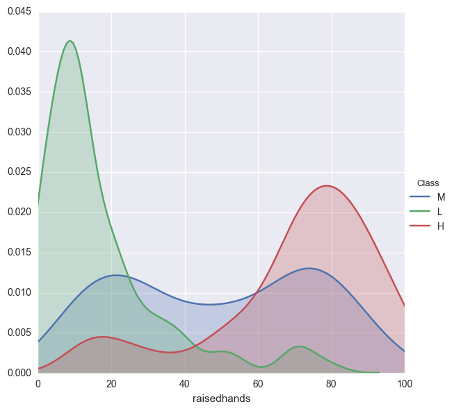
As suspected, students that perform poorly rarely raise their hands, while students that perform okay have a greater variation of participation. Something to consider may be that the poorly performing students can not raise their hand because they are absent from class.
Check out discussion group participation across classes
facetgrid = sns.FacetGrid(edu,hue='Class',size=6)
facetgrid.map(sns.kdeplot,'Discussion',shade=True)
facetgrid.set(xlim=(0,edu['Discussion'].max()))
facetgrid.add_legend();
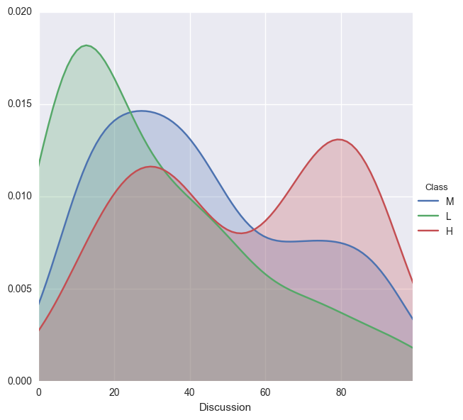
Both low and middle performing students do not go to the discussion groups very often. However, the high performing students fall in to two catgories: those goody two shoes that go to a bunch of discussions, and those that go to a decent amount.
Take a look at the topics:
sns.countplot(x = "Topic", data = edu, hue = 'Class', palette = "muted");
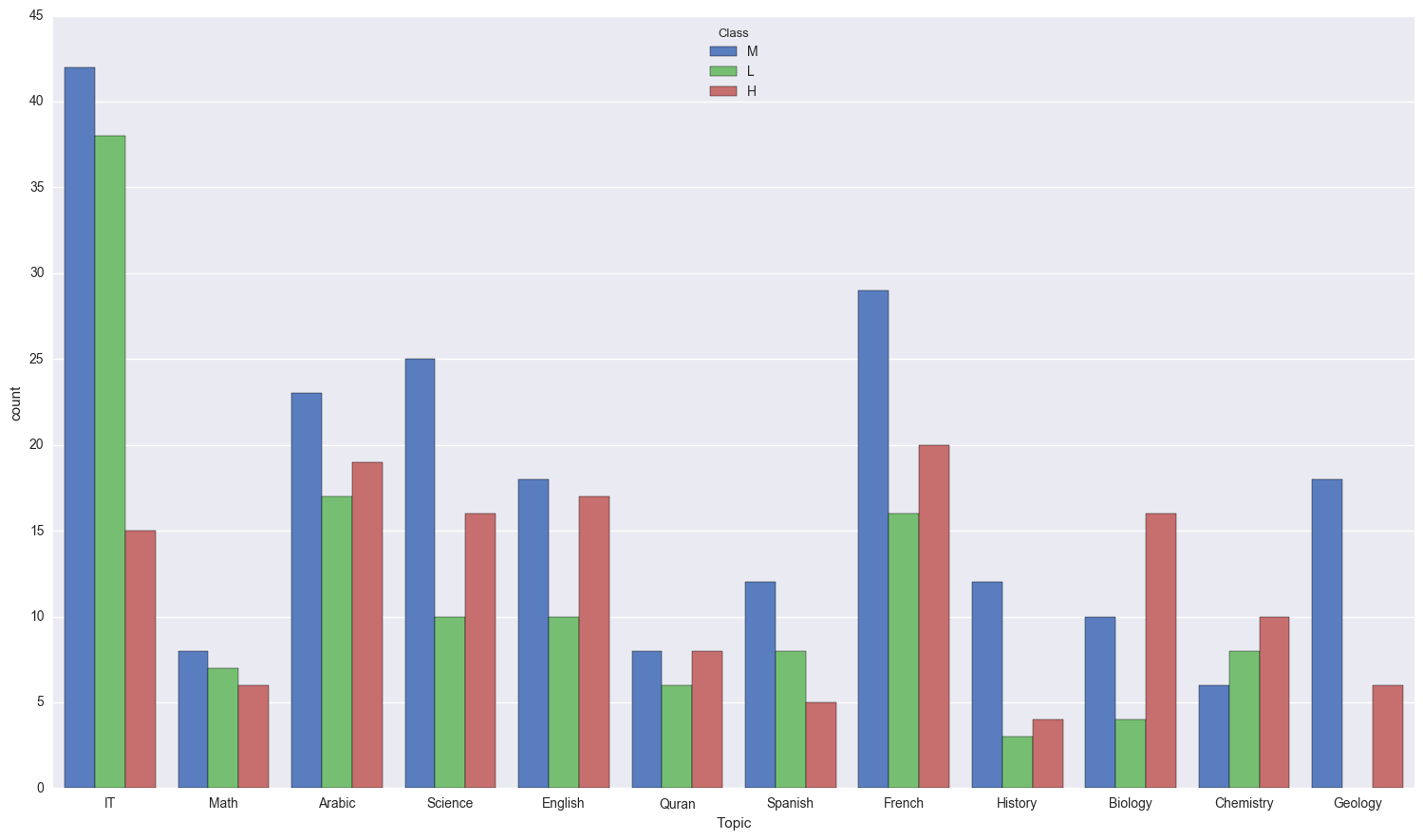
A LOT of students didn’t do so hot in IT, however lets take a deeper look in to the relative amounts of students for each topic that didn’t do well.
pd.crosstab(edu.Class, edu.Topic, normalize = 'columns')
| Topic | Arabic | Biology | Chemistry | English | French | Geology | History | IT | Math | Quran | Science | Spanish |
|---|---|---|---|---|---|---|---|---|---|---|---|---|
| Class | ||||||||||||
| H | 0.322034 | 0.533333 | 0.416667 | 0.377778 | 0.307692 | 0.25 | 0.210526 | 0.157895 | 0.285714 | 0.363636 | 0.313725 | 0.20 |
| L | 0.288136 | 0.133333 | 0.333333 | 0.222222 | 0.246154 | 0.00 | 0.157895 | 0.400000 | 0.333333 | 0.272727 | 0.196078 | 0.32 |
| M | 0.389831 | 0.333333 | 0.250000 | 0.400000 | 0.446154 | 0.75 | 0.631579 | 0.442105 | 0.380952 | 0.363636 | 0.490196 | 0.48 |
A full 40% of students failed their IT class… that’s brutal. Tied for second place are Math and Chemistry at 1/3 of students.
Classification
Time to get down to business and do some predictions. First, I need to do some data massaging to get it all in to a usable format. I will one hot endcode gender, student absence days and topics. Then, I will split the data in to training and testing groups. Then, I will optimize my classifiers.
A note about sklearn’s gridsearch, xgboost and parellization
After fighting for hours with gridsearch and xgboost and trying to get gridsearch to work with multiple threads, I have finally figured out what was wrong.
The Problem: Xgboost automatically does multithreading (nthread = -1), so that it uses all of your computer’s cores. However, when you try and combine that with gridsearch’s multithreading, they don’t play nicely. The gridsearch will initially work, but after a couple of seconds all of the threads will hang and do nothing. This is extremely frustrating as using only 1 thread could literally take days (especially on such a small dataset!).
The Solution: Let gridsearch do it’s thing. Set the nthread parameter in xgboost to 1 so that it only uses 1 thread. When you instantiate your gridsearch instance, set n_jobs = -1. This will allow gridsearch to fully control the threading so that you don’t have two different packages fighting for control of threads.
edu['gender'] = edu.gender.apply(lambda x : 1 if x == "M" else 0)
edu['StudentAbsenceDays'] = edu.StudentAbsenceDays.apply(lambda x : 1 if x == 'Above-7' else 0)
edu = edu.join(pd.get_dummies(edu.Topic))
x = edu[['const','gender', 'raisedhands', 'VisITedResources', 'AnnouncementsView', 'Discussion', 'StudentAbsenceDays',
         'ParentschoolSatisfaction', 'Arabic', 'Biology', 'Chemistry', 'English', 'French', 'Geology',
         'History', 'IT', 'Math', 'Quran', 'Science', 'Spanish' ]]
y = edu.Class

def get_int_cat(y):
    if y == 'H':
        return 2
    elif y == 'M':
        return 1
    else:
        return 0
y = y.apply(get_int_cat)
x_train, x_test, y_train, y_test = train_test_split(x, y, test_size = 0.3)

x_train.columns.values, x_test.columns.values
(array(['const', 'gender', 'raisedhands', 'VisITedResources',
        'AnnouncementsView', 'Discussion', 'StudentAbsenceDays',
        'ParentschoolSatisfaction', 'Arabic', 'Biology', 'Chemistry',
        'English', 'French', 'Geology', 'History', 'IT', 'Math', 'Quran',
        'Science', 'Spanish'], dtype=object),
 array(['const', 'gender', 'raisedhands', 'VisITedResources',
        'AnnouncementsView', 'Discussion', 'StudentAbsenceDays',
        'ParentschoolSatisfaction', 'Arabic', 'Biology', 'Chemistry',
        'English', 'French', 'Geology', 'History', 'IT', 'Math', 'Quran',
        'Science', 'Spanish'], dtype=object))
init_xgb = XGBClassifier(objective = 'multi:softmax', nthread = 1) #nthread = 1, as noted above
init_xgb.fit(x_train, y_train)
pred = init_xgb.predict(x_test)
print classification_report(y_test, pred)
             precision    recall  f1-score   support

          0       0.82      0.94      0.87        33
          1       0.65      0.72      0.68        64
          2       0.69      0.51      0.59        47

avg / total       0.70      0.70      0.69       144
param_list = init_xgb.get_params()
def tune_w_GS(testing_params, estimator, data, predictors, target, n_folds = 3):
    print predictors

    gsearch = GridSearchCV(estimator, param_grid = testing_params, n_jobs = -1, verbose = 1,
                          cv= n_folds)

    gsearch.fit(data[predictors], data[target])

    gsearch.grid_scores_
    print gsearch.best_params_
    print gsearch.best_score_

    return gsearch
print param_list
{'reg_alpha': 0, 'colsample_bytree': 1, 'silent': True, 'colsample_bylevel': 1, 'scale_pos_weight': 1, 'learning_rate': 0.1, 'missing': None, 'max_delta_step': 0, 'nthread': 1, 'base_score': 0.5, 'n_estimators': 100, 'subsample': 1, 'reg_lambda': 1, 'seed': 0, 'min_child_weight': 1, 'objective': 'multi:softprob', 'max_depth': 3, 'gamma': 0}
x_train.columns.values
array(['const', 'gender', 'raisedhands', 'VisITedResources',
       'AnnouncementsView', 'Discussion', 'StudentAbsenceDays',
       'ParentschoolSatisfaction', 'Arabic', 'Biology', 'Chemistry',
       'English', 'French', 'Geology', 'History', 'IT', 'Math', 'Quran',
       'Science', 'Spanish'], dtype=object)
#try 3 different max_depths, and 3 different child weights
param_test1 = {
     'max_depth'        : [3,4],
     'reg_alpha'        : [0, 0.5, 1, 1.5],
     'colsample_bytree' : [0.9, 1],
     'learning_rate'    : [.005, .01, .015, .02, .05, .1, .15],
     'n_estimators'     : [100, 500, 750, 1000],
     'gamma'            : [0, .05, .1, 0.15]

}

# 'max_delta_step'   : [0, 0.05, 0.1, 0.3],
#     'n_estimators'     : [100, 500, 750, 1000],
#     'subsample'        : [i/10.0 for i in range(6,11)],
#     'reg_lambda'       : [.5, 1, 1.5, 2],
#     'min_child_weight' : range(1,6,2),
#     'max_depth'        : range(3,7),
#     'gamma'            : [i/100.0 for i in range(0,30, 5)]

gsearch = tune_w_GS(param_test1, estimator = XGBClassifier(**param_list), data = edu,
                    predictors = list(x_train.columns.values), target = 'Class', n_folds = 4)


gsearch.best_params_, gsearch.best_score_
['const', 'gender', 'raisedhands', 'VisITedResources', 'AnnouncementsView', 'Discussion', 'StudentAbsenceDays', 'ParentschoolSatisfaction', 'Arabic', 'Biology', 'Chemistry', 'English', 'French', 'Geology', 'History', 'IT', 'Math', 'Quran', 'Science', 'Spanish']
Fitting 4 folds for each of 1792 candidates, totalling 7168 fits


[Parallel(n_jobs=-1)]: Done  52 tasks      | elapsed:    5.7s
[Parallel(n_jobs=-1)]: Done 210 tasks      | elapsed:   20.0s
[Parallel(n_jobs=-1)]: Done 460 tasks      | elapsed:   45.2s
[Parallel(n_jobs=-1)]: Done 810 tasks      | elapsed:  1.2min
[Parallel(n_jobs=-1)]: Done 1260 tasks      | elapsed:  1.9min
[Parallel(n_jobs=-1)]: Done 1810 tasks      | elapsed:  2.7min
[Parallel(n_jobs=-1)]: Done 2460 tasks      | elapsed:  3.8min
[Parallel(n_jobs=-1)]: Done 3210 tasks      | elapsed:  5.0min
[Parallel(n_jobs=-1)]: Done 4060 tasks      | elapsed:  6.4min
[Parallel(n_jobs=-1)]: Done 5010 tasks      | elapsed:  7.9min
[Parallel(n_jobs=-1)]: Done 6060 tasks      | elapsed:  9.6min
[Parallel(n_jobs=-1)]: Done 7168 out of 7168 | elapsed: 11.6min finished


{'reg_alpha': 0, 'colsample_bytree': 1, 'learning_rate': 0.02, 'n_estimators': 500, 'max_depth': 4, 'gamma': 0}
0.670833333333


/Users/benjamindykstra/anaconda/lib/python2.7/site-packages/sklearn/model_selection/_search.py:667: DeprecationWarning: The grid_scores_ attribute was deprecated in version 0.18 in favor of the more elaborate cv_results_ attribute. The grid_scores_ attribute will not be available from 0.20
  DeprecationWarning)


({'colsample_bytree': 1,
  'gamma': 0,
  'learning_rate': 0.02,
  'max_depth': 4,
  'n_estimators': 500,
  'reg_alpha': 0},
 0.67083333333333328)
param_list = gsearch.best_estimator_.get_params()

xgb2 = XGBClassifier(**param_list)
xgb2.fit(x_train, y_train)
pred = xgb2.predict(x_test)

print "Classification Report: \n"
print classification_report(y_test, pred)
print('Accuracy: %.2f' % accuracy_score(y_test, pred))
Classification Report:

             precision    recall  f1-score   support

          0       0.79      0.94      0.86        33
          1       0.63      0.69      0.66        64
          2       0.66      0.49      0.56        47

avg / total       0.68      0.68      0.67       144

Accuracy: 0.68
Neural Net tuning for predictions
just using a simple sequential model with a couple of layers
import keras
from keras.models import Sequential
from keras.wrappers.scikit_learn import KerasClassifier
from keras.layers import Dense, Activation, Dropout
from sklearn.preprocessing import StandardScaler, MinMaxScaler
from sklearn.cross_validation import StratifiedKFold, cross_val_score, train_test_split
from sklearn.pipeline import Pipeline
from sklearn.metrics import confusion_matrix, classification_report
from keras.utils.np_utils import to_categorical
Using Theano backend.
class LossHistory(keras.callbacks.Callback):
    """Tracks loss and accuracy per batch"""
    def on_train_begin(self, logs={}):
        self.losses = []
        self.acc = []

    def on_batch_end(self, batch, logs={}):

        self.losses.append(logs.get('loss'))
        self.acc.append(logs.get('acc'))
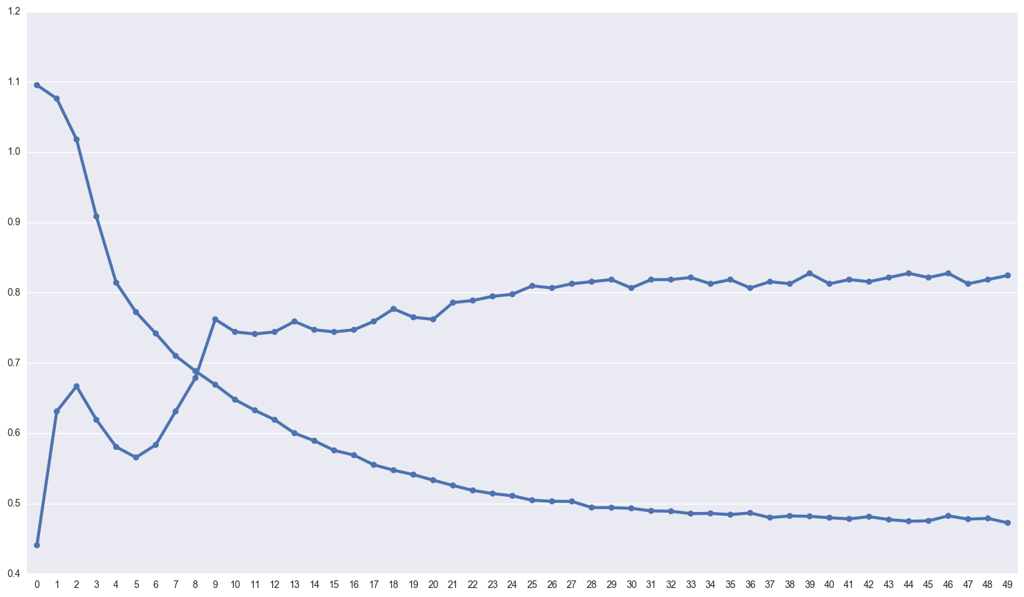
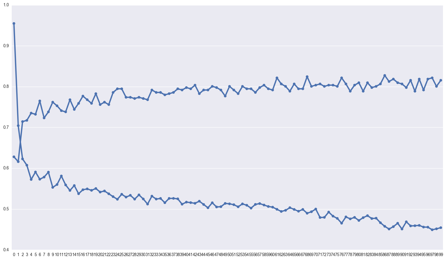
def plot_history(history):
    if isinstance(history, LossHistory):
        hist_dict = {}
        losses = np.asarray(history.losses)
        acc = np.asarray(history.acc)
        avg_loss, avg_acc = [], []
        sub_loss, sub_acc = [], []
        for i in xrange(losses.size):

            if i % 100 == 0 and i != 0:
                avg_loss.append(np.asarray(sub_loss).mean())
                avg_acc.append(np.asarray(sub_acc).mean())
                sub_loss, sub_acc = [], []
            else:
                sub_loss.append(losses[i])
                sub_acc.append(acc[i])

        hist_dict['loss'] = np.asarray(avg_loss)
        hist_dict['acc'] = np.asarray(avg_acc)
    else:
        hist_dict = history.history
    fig, ax = plt.subplots()
    fig.set_size_inches(18.5, 10.5)
    sns.pointplot(x = range(len(hist_dict['loss'])), y = hist_dict['loss'], markers = '.', ax = ax);
    sns.pointplot(x = range(len(hist_dict['loss'])), y = hist_dict['acc'], markers = '.', ax = ax);
def performance(model, x_test, y_true):

    pred = model.predict(x_test)

    print "The classification_report: "
    print classification_report(y_true, pred)
Inputs to keras models must be numpy arrays, they cannot be dataframes. Additionally, the target variable, in this case ‘Class’ must be one hot encoded for the multiclass case.
dummy_y_train = pd.get_dummies(y_train).values
type(dummy_y_train)
numpy.ndarray
dummy_y_train
array([[0, 1, 0],
       [0, 1, 0],
       [0, 1, 0],
       ...,
       [0, 1, 0],
       [1, 0, 0],
       [0, 1, 0]], dtype=uint8)
Properly scale the data. Neural nets are sensitive to the scale of input data.
sc = StandardScaler()
x_train_std = sc.fit_transform(x_train)
x_test_std = sc.transform(x_test)
type(x_train_std)
numpy.ndarray
def create_baseline():
    model = Sequential()
    model.add(Dense(65, input_dim=20, init='normal', activation='tanh'))
    model.add(Dense(32, init='normal', activation='tanh'))
    model.add(Dense(16, init= 'normal', activation = 'tanh'))
    model.add(Dense(3, init='normal', activation='softmax'))

    model.compile(loss='categorical_crossentropy', optimizer='adam', metrics=['accuracy'])
    return model
estimator = KerasClassifier(build_fn=create_baseline, nb_epoch = 50, verbose=0)
history = estimator.fit(x_train_std, dummy_y_train)
y_test_pred = estimator.predict(x_test_std)

print classification_report(y_test, y_test_pred)
plot_history(history)
             precision    recall  f1-score   support

          0       0.77      0.91      0.83        33
          1       0.69      0.67      0.68        64
          2       0.72      0.66      0.69        47

avg / total       0.72      0.72      0.72       144
estimator.score(x_train_std, y_train)
0.83333333333333337
estimator.score(x_test_std, y_test)
0.72222222222222221
def create_larger():
    model = Sequential()
    model.add(Dense(output_dim = 64, input_dim = 20, init = 'normal', activation = 'tanh'))
    model.add(Dense(output_dim = 128, init = 'normal', activation = 'tanh'))
    model.add(Dense(output_dim = 256, init = 'normal', activation = 'tanh'))
    model.add(Dense(output_dim = 256, init = 'normal', activation = 'tanh'))
    #model.add(Dropout(0.2))
    model.add(Dense(output_dim = 128,  init = 'normal', activation = 'tanh'))
#     model.add(Dense(output_dim = 64,  init = 'normal', activation = 'tanh'))
#     model.add(Dense(output_dim = 32, init = 'normal', activation = 'relu'))
    model.add(Dense(output_dim = 3, init = 'normal', activation = 'softmax'))
    #opt = keras.optimizers.Adam(lr=0.001, beta_1=0.9, beta_2=0.999, epsilon=1e-08)
    model.compile(loss = 'categorical_crossentropy', optimizer = 'adadelta', metrics = ['accuracy'])
    return model
large_estimator = KerasClassifier(build_fn=create_larger, nb_epoch = 100, batch_size = 20, verbose=0)
history = large_estimator.fit(x_train_std, dummy_y_train)
y_test_pred = large_estimator.predict(x_test_std)

print classification_report(y_test, y_test_pred)

plot_history(history)
             precision    recall  f1-score   support

          0       0.76      0.97      0.85        33
          1       0.71      0.66      0.68        64
          2       0.72      0.66      0.69        47

avg / total       0.73      0.73      0.72       144
Gridsearch for the neural net
Beware, this code took 13 hours to finish on my machine
# def create_larger_grid(activation = 'tanh', initialization = 'normal', dropout = 0.0, optimizer = 'adam'):
#     model = Sequential()
#     model.add(Dense(output_dim = 64, input_dim = 19, init = initialization, activation = 'tanh'))
#     model.add(Dense(output_dim = 128, init = initialization, activation = 'tanh'))
#     model.add(Dense(output_dim = 256, init = initialization, activation = 'tanh'))
#     model.add(Dense(output_dim = 256, init = initialization, activation = 'tanh'))
#     model.add(Dropout(dropout))
#     model.add(Dense(output_dim = 128,  init = initialization, activation = 'tanh'))
#     model.add(Dense(output_dim = 64,  init = initialization, activation = 'tanh'))
#     model.add(Dense(output_dim = 3, init = initialization, activation = 'softmax'))
#     #opt = keras.optimizers.Adam(lr=0.001, beta_1=0.9, beta_2=0.999, epsilon=1e-08)
#     model.compile(loss = 'categorical_crossentropy', optimizer = optimizer, metrics = ['accuracy'])
#     return model


# model = KerasClassifier(build_fn=create_larger_grid, verbose=0)

# batch_size = [10, 20, 40, 60]
# epochs = [50, 150]
# algs = ['SGD', 'RMSprop', 'Adagrad', 'Adadelta', 'Adam', 'Adamax', 'Nadam']
# init_options =  ['uniform',  'normal', 'glorot_normal', 'glorot_uniform']
# act_fns = ['softmax', 'softplus', 'softsign', 'relu', 'tanh', 'sigmoid', 'hard_sigmoid', 'linear']
# drop = [0.0, 0.1, 0.2, 0.3, 0.4]
# param_grid = dict(batch_size = batch_size, nb_epoch = epochs, optimizer = algs, initialization = init_options,
#                   activation = act_fns, dropout = drop)

# start = time.time()

# grid = GridSearchCV(estimator=model, param_grid=param_grid, n_jobs = -1)
# grid_result = grid.fit(x_train_std, dummy_y_train)

# elapsed = time.time() - start

# print "Elapsed time for big gridsearch: ", elapsed
# # summarize results
# print "Best: %f using %s" % (grid_result.best_score_, grid_result.best_params_)

# """
#     Best: 0.732143 using {'optimizer': 'Adam', 'initialization': 'glorot_normal',
#     'batch_size': 40, 'activation': 'softsign', 'nb_epoch': 50, 'dropout': 0.2}
# """
Replicating that model below, for some reason passing in params works with gridsearch, does not work passing in params directly to the model.
def create_larger_grid():
    model = Sequential()
    model.add(Dense(output_dim = 64, input_dim = 20, init = 'glorot_normal', activation = 'softsign'))
    model.add(Dense(output_dim = 128, init = 'glorot_normal', activation = 'softsign'))
    model.add(Dense(output_dim = 256, init = 'glorot_normal', activation = 'softsign'))
    model.add(Dropout(0.1))
    model.add(Dense(output_dim = 256, init = 'glorot_normal', activation = 'softsign'))
    model.add(Dropout(0.2))
    model.add(Dense(output_dim = 256, init = 'glorot_normal', activation = 'softsign'))
    model.add(Dense(output_dim = 128, init = 'glorot_normal', activation = 'softsign'))
    model.add(Dropout(0.2))
    model.add(Dense(output_dim = 64,  init = 'glorot_normal', activation = 'softsign'))
    model.add(Dense(output_dim = 32,  init = 'glorot_normal', activation = 'softsign'))
    model.add(Dense(output_dim = 3, init = 'glorot_normal', activation = 'softmax'))
    #opt = keras.optimizers.Adam(lr=0.001, beta_1=0.9, beta_2=0.999, epsilon=1e-08)
    model.compile(loss = 'categorical_crossentropy', optimizer = 'adam', metrics = ['accuracy'])
    return model
         precision    recall  f1-score   support

      0       0.74      0.88      0.81        33
      1       0.87      0.45      0.59        73
      2       0.55      0.97      0.70        38
avg / total 0.76 0.69 0.67 144
params =  {'optimizer': 'Adam', 'initialization': 'glorot_normal', 'activation': 'softsign', 'dropout': 0.2}
best_model = KerasClassifier(build_fn = create_larger_grid,batch_size = 40, nb_epoch = 100, verbose = 0)

history = best_model.fit(x_train_std, dummy_y_train)


performance(best_model, x_test_std, y_test)
plot_history(history)
The classification_report:
             precision    recall  f1-score   support

          0       0.77      0.91      0.83        33
          1       0.70      0.67      0.69        64
          2       0.73      0.68      0.70        47

avg / total       0.73      0.73      0.73       144
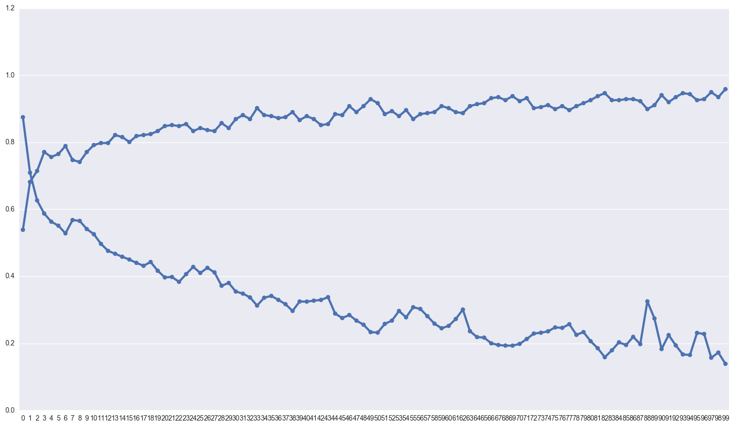
My suspicion is that the model is overfitting pretty badly, which is why I’ve added so much dropout. Lets take a look at the difference between the scores on the training and test sets.
best_model.score(x_train_std, y_train)
0.9583333304950169
best_model.score(x_test_std, y_test)
0.72916666997803581
KNN and Logistic Classifiers
from sklearn.neighbors import KNeighborsClassifier
knn = KNeighborsClassifier()

knn.fit(x_train, y_train)

knn_pred = knn.predict(x_test)

performance(knn, x_test, y_test)
The classification_report:
             precision    recall  f1-score   support

          0       0.61      0.91      0.73        33
          1       0.60      0.56      0.58        64
          2       0.66      0.49      0.56        47

avg / total       0.62      0.62      0.61       144
logit = LogisticRegression(multi_class='multinomial', solver = 'newton-cg')
logit.fit(x_train, y_train)

logit_pred = logit.predict(x_test)

performance(logit,x_test, y_test)
The classification_report:
             precision    recall  f1-score   support

          0       0.79      0.94      0.86        33
          1       0.67      0.70      0.69        64
          2       0.71      0.57      0.64        47

avg / total       0.71      0.72      0.71       144
logit.score(x_train, y_train), logit.score(x_test,y_test)
(0.7857142857142857, 0.71527777777777779)
Wow, the logistic regression is destroying the competition here, with the test set score almost exactly the same as the neural net.
from mlxtend.classifier import EnsembleVoteClassifier
from sklearn.model_selection import cross_val_score
eclf = EnsembleVoteClassifier(clfs=[xgb2, logit, knn], voting = 'soft', weights=[0.25,0.5,0.25])

labels = ['boosted tree', 'logit', 'k-nearest neighbors', 'Ensemble']

for clf, label in zip([xgb2, logit, knn, eclf], labels):

    scores = cross_val_score(clf, x, y,cv=5,scoring='accuracy')
    print("Accuracy: %0.2f (+/- %0.2f) [%s]"
          % (scores.mean(), scores.std(), label))
Accuracy: 0.64 (+/- 0.07) [boosted tree]
Accuracy: 0.64 (+/- 0.07) [logit]
Accuracy: 0.60 (+/- 0.04) [k-nearest neighbors]
Accuracy: 0.65 (+/- 0.03) [Ensemble]
Cross validated score of the neural net
from sklearn.metrics import precision_recall_fscore_support

def load_data():
    return edu, edu.columns.values

def create_model():
    return KerasClassifier(build_fn = create_larger_grid,batch_size = 40, nb_epoch = 100, verbose = 0)

def train_and_evaluate__model(model, x_train, y_train, x_test, y_test):
    history = model.fit(x_train, dummy_y_train)
    pred = model.predict(x_test)
    p,r,fb,s = precision_recall_fscore_support(y_test, pred)
    return model.score(x_test, y_test), p,r,fb,s
from sklearn.model_selection import StratifiedKFold
from sklearn.metrics import precision_recall_fscore_support

data, labels = load_data()
n_folds = 10
skf = StratifiedKFold(n_splits=n_folds, shuffle=True)

all_scores =[]
all_p = []
all_r = []
for train_index, test_index in skf.split(x, y):
    x_train, x_test = x.ix[train_index], x.ix[test_index]
    y_train, y_test = y[train_index], y[test_index]
    sc = None
    sc = StandardScaler()
    x_train_std = sc.fit_transform(x_train)
    x_test_std = sc.transform(x_test)
    dummy_y_train = pd.get_dummies(y_train).values

    model = None
    model = create_model()
    score, p,r,fb,s = train_and_evaluate__model(model,x_train_std, dummy_y_train, x_test_std, y_test)
    all_scores.append(score)
    all_p.append(p)
    all_r.append(r)

print("Accuracy of neural net: %0.2f (+/- %0.2f) " % (np.array(all_scores).mean(), np.array(all_scores).std()))

for i in xrange(0,3):
    print("Precision for class %d: %0.2f (+/- %0.2f) " % (i, np.array(all_p)[:,i].mean(), np.array(all_p)[:,i].std()))
    print("   Recall for class %d: %0.2f (+/- %0.2f) " % (i,np.array(all_r)[:,i].mean(), np.array(all_r)[:,i].std()))
Accuracy of neural net: 0.73 (+/- 0.07)
Precision for class 0: 0.85 (+/- 0.11)
   Recall for class 0: 0.84 (+/- 0.13)
Precision for class 1: 0.70 (+/- 0.07)
   Recall for class 1: 0.71 (+/- 0.09)
Precision for class 2: 0.71 (+/- 0.10)
   Recall for class 2: 0.67 (+/- 0.11)
In the end, the neural net still outperforms the ensembling of the other methods. The standard deviation of the precision and recall are rather high and it would be better if they were lower. We were able to pretty accurately identify low performing students, however high performing students were a bit harder to distinguish from the middle performing students.
I was able to use an ensemble classifier to improve the performance of a KNN classifier, xgboost and a logistic regression. The ensemble classifier did not outperform the tuned feed forward neural net. The tradeoff to using the network is the lack of interpretability that could be gleaned from say a logistic regression model.
Thanks for following along again :) Hit me up at bfdykstra@email.wm.edu for questions/comments/suggestions